Occasionally we hear about a famous museum heist, and maybe we wonder how it was done. I can’t explain how the criminals could get past all the security measures in museums, but I can offer some insight as to how criminals might choose what to take. And although scheduling vehicles and drivers is pretty different from planning a museum heist, the greedy mind of a criminal can still teach us a thing or two about schedule optimization.
Picture this: You are burglarizing a museum and plan to steal many priceless artifacts from their collections. You only have your backpack to put things in, and since you haven’t been to the gym in a while, you can’t carry more than 50 pounds while you run away. You want to take as many highly valued items as you can, so you need to figure out how to yield the highest value without surpassing your 50-pound weight limit. These are your options:
| Item | Value ($) | Weight (lbs) |
|---|---|---|
| Fossils | 4,340 | 25 |
| Plaque | 330 | 9 |
| Pearl necklace | 1,950 | 7 |
| Marble sculpture | 2,290 | 9 |
| Silver coins | 3,700 | 8 |
| Cash | 3,030 | 4 |
| Block of gold | 4,620 | 11 |
| Museum tickets | 160 | 1 |
| Ancient scroll | 2,780 | 1 |
| Crown | 4,810 | 13 |
Before you continue reading, think about how you would figure out which items to take with you. (Hint: you can sort the items by value and cost/weight!)
This scenario is an example of the knapsack problem, a simple scenario that can be solved with optimization.
You select the crown, block of gold, fossils, and ancient scroll, reaching a total value of $16,550. Wondering if you can do better than that, you take everything out and start over, but this time you select according to the artifacts that weigh the least. Now, your backpack contains the museum tickets, an ancient scroll, cash, a pearl necklace, silver coins, a plaque, a marble sculpture, and a block of gold, totaling $18,860 in value. You are content with the higher value and quickly run away before you are caught.
The mechanism you used to decide which items to take is called the greedy algorithm, a fundamental concept in understanding optimization. In fact, if you had used the greedy algorithm according to value-density (value ÷ cost), you would have achieved an even higher total value, at $21,050. But this would not be the case in every scenario, nor is it the highest possible value that you could have stolen from the museum.
| Greedy Parameter | Algorithm Outcome | Total Value |
|---|---|---|
| Value | Crown, block of gold, fossils, ancient scroll | $16,550 |
| Cost (Weight) | Museum tickets, ancient scroll, cash, pearl necklace, silver coins, plaque, marble sculpture, block of gold | $18,860 |
| Density (Cost/Value) | Ancient scroll, cash, silver coins, block of gold, crown, pearl necklace, museum tickets | $21,050 |
Here’s what the code for the greedy algorithm would look like in Python:
Using the greedy algorithm for large optimization problems will give us a local maximum, but it will rarely yield a global maximum.
It’s like if you were to reach the peak of a mountain, without seeing that another mountain in the distance is even taller than the one you are on. In order to find the global, or absolute, maximum value, we would need to examine every possible scenario.
We can do this using a recursive program that works like a search tree. For each item we could potentially take with us, we will look at the total value we would get if we take the item, versus if we do not take the item. The diagram below illustrates a simplified version of the problem, using only 3 items.
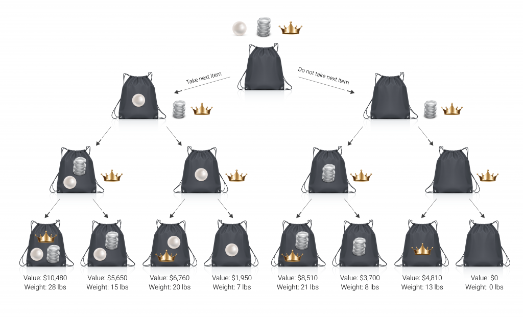
Since we are only including three items in this simplified example (the pearls, the silver, and the crown), imagine your weight limit is 25 pounds. Which items would you take?
In this case, taking all three items will obviously yield the highest profit, but it goes over your weight limit. The next best plan is to take the crown and silver coins, because you will maximize profit without surpassing 25 lbs.
Here is what the code looks like for this “branching” optimization method:
This branching algorithm would yield an even better outcome than the greedy algorithm does.
The optimal choice for the thief would have been to take the crown, ancient scroll, museum tickets, block of gold, cash, silver coins, and marble sculpture, and have a total value of $21,390.
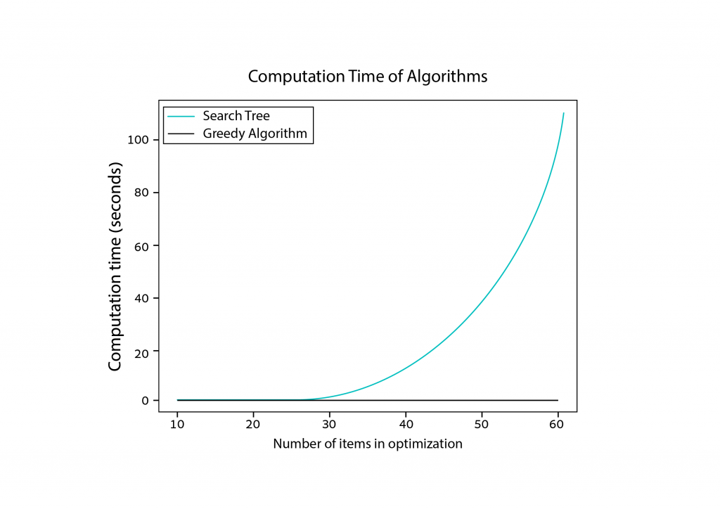
As you can see in the diagram above, the problem gets really complex, really fast! A computer can easily solve the problem with 10 items in less than a second, but when there are 50 items it takes a few seconds, and with 70 items it takes more than 10 minutes on average! True optimization is np-hard, meaning that the difficulty of solving it (i.e. the time it takes) increases drastically as the problem size increases. On the other hand, the greedy algorithm remains stable in comparison, taking a few milliseconds. It’s no wonder a burglar would want to use the greedy algorithm, as it would save them a lot of time.
But, there’s a tradeoff.
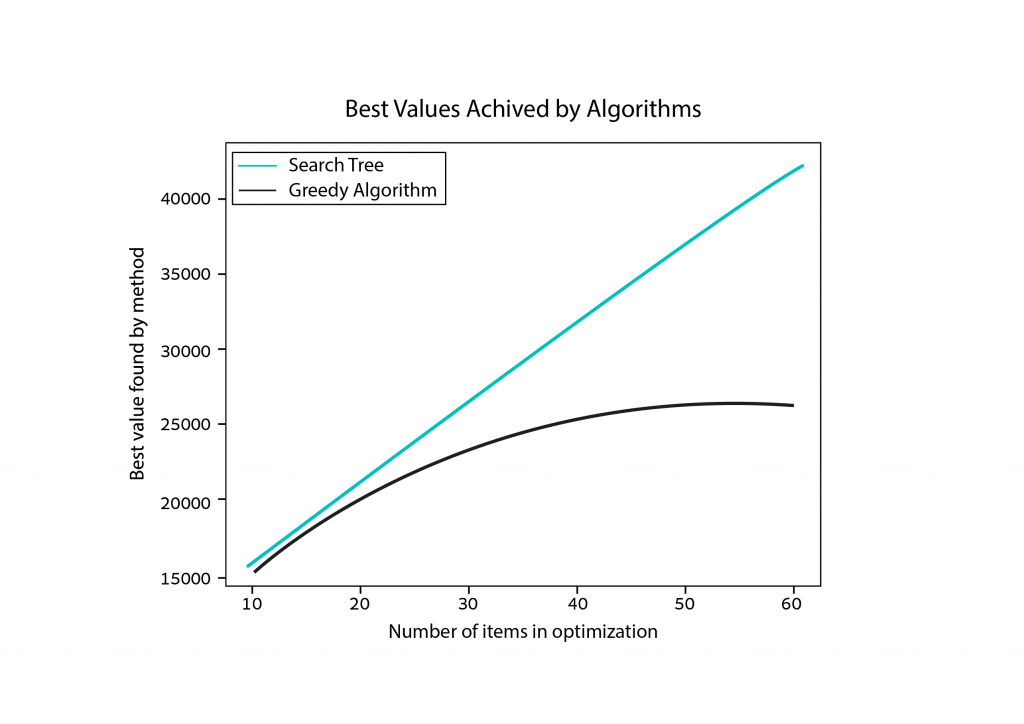
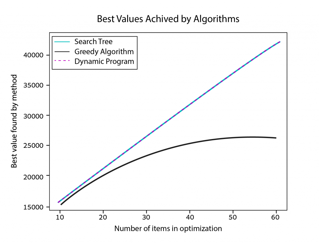
We already knew that the greedy algorithm doesn’t always give the best solution, but it did get pretty close in the last example. In the chart below, we can see that as the size of the problem increases, so does the disparity in the optimal values that each method achieves.
Is there another more efficient optimization strategy?
In the backpack diagram above, notice how many of the branches, or sub-problems, look similar to one another. Dynamic programming — an advanced optimization strategy — saves computing power by storing the results of these sub-problems for later use (via a process called memoization). It turns out that this approach saves a whole lot of time! And since dynamic programming algorithms follow the search tree structure, the results will always be optimal. With dynamic programming, we can compute optimal results in a timeframe closer to that of the greedy algorithm. See for yourself in the charts below.

So, what can a burglar teach us about building schedules?
In a way, transportation planning problems are similar to the knapsack problem. When we plan a city’s transportation network and optimize its operations, we are choosing routes and trips for each vehicle and driver under a set of constraints, similar to how the burglar chooses items to steal from the museum.
In real life, however, the problem is much more complex. First, we have many “burglars”; in a sense, all vehicles and drivers make up a team of burglars, and we want to optimize each of their individual operations to get the best-combined outcome. Second, real-life constraints are much more complicated because we are dealing with people and uncertainty. For example, we might have a constraint where a driver needs a 30-minute break in a specific location at least every 4 working hours. On top of this, in real life, trips might run late, so accounting for trip delays in the planning process can improve on-time performance and avoid service penalties.
The burglar wants to solve his optimization problem as fast as possible, and so does Optibus — but we aren’t willing to settle for the “greedy” solution.
As with the knapsack problem, these transportation planning problems are NP-hard and require a large arsenal of advanced heuristics and algorithms to properly solve.
When solving large-scale vehicle and crew scheduling problems we must take into account a wide set of trade-offs and constraints such as operating costs, on-time performance, labor laws, and other regulations. In order to reach the best solution, we must consider lots of different variables and examine many different possible outcomes.
At Optibus, we use a combination of graph theory-related algorithms, machine learning, and AI algorithms to solve these transportation optimization problems on the cloud. This way, we can solve problems in a distributed way, taking advantage of massive cloud resources and serverless computing. This allows us to plan the operation of large scale transportation networks in a very short time —as if we were just solving a simple knapsack problem.